
Stratified estimation of area and accuracy ✓
An example is provided here to illustrate the estimation of the area of forest loss for the country of Cambodia between 2000 and 2010 using stratified estimation. The example has three different parts: 1) sampling design – a sample is selected by stratified random sampling; 2) response design which involves observing the reference conditions at sample unit in various satellite data available in Google Earth Engine; and 3) the analysis which is based on the application of a stratified estimator to the sample data.
Note that the sample data are made-up and do not reflect actual conditions in Cambodia!
1. Sampling Design
- Stratification. Because the area of forest loss is small relative the total study area, using non-stratified designs would require a very large sample size to ensure a sufficient number of observations of forest loss in the sample data. To use a stratified design, we will first need to define a stratification. In this case, we will extract a map of Cambodia from a global map [1] of (1) forest, (2) non-forest, (3) water, (4) forest loss, (5) forest gain, and (6) forest loss and gain. The map will serve a stratification of study area. Preferably, use the GeoTIFF format. (A tutorial from BEEODA illustrating the creation of a local stratification from the global map is provided here)
- You can download the stratification of Cambodia here. Once downloaded to your local computer, click the Assets tab next to the Scripts tab and NEW > Image upload > SELECT; click Advanced > Masking mode > and set No-data value to “0”. Click OK to upload the stratification as an image file. You can check the progress in the Tasks tab (the upload will take several minutes).
- Once the stratification has been added to Assets, highlight the script “1_Sampling_Design” in the Scripts tab and click Run. (Check Overview to familiarize yourself with GEE interface if you have done so already.)
- In Sampling Design dialog, click Stratified or Simple Random Sampling > add the path to the stratification under Specify an image to define study area. The path is likely something like “users/[your name]/stratification_cambodia_utm_small”. Set the band to “1” and mask value to “0” and click Load image.
- Sampling scheme. Because the objective of the exercise is to estimate the area forest loss which is a small part of the study area, the sample will be selected by stratified random sampling – under Select a sampling scheme select Stratified random.
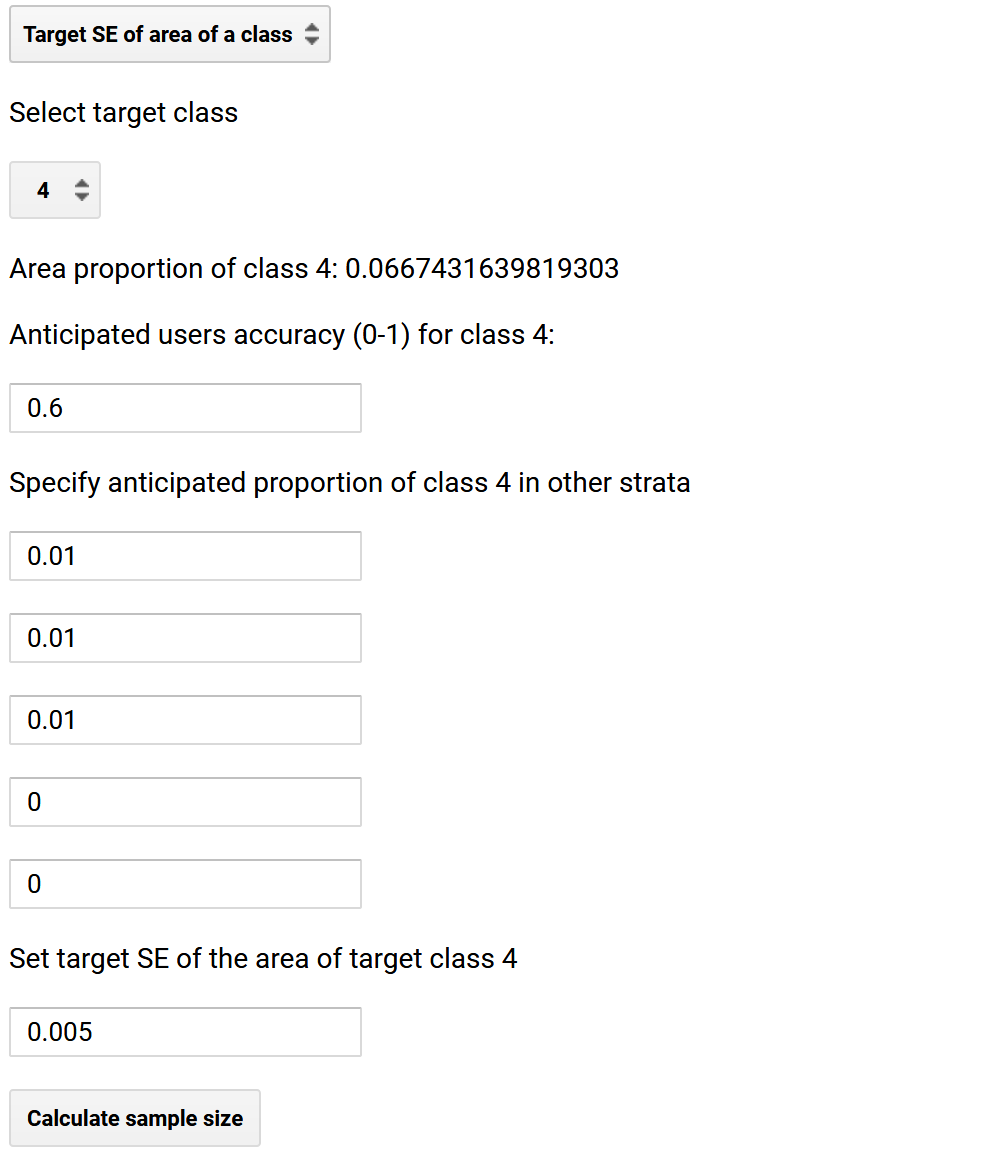
- Sample size. Further, we will Determine sample size by setting a Target SE of a class, in this case, class number 4, Forest loss. The application will print in the Dialog and Console the area proportion of class 4:
>>> Area proportion of class 4:
    0.0667431639819303
- To determine the sample size, n, we’ll use Equation 5.25 in [2]
where \(W_h\) are the strata weights that are automatically extracted from the stratification; \(\mbox{SD}_h\) are the stratum standard deviations, calculated as \(\mbox{SD}_h= \sqrt{p_h (1-p_h)}\) where \(p_h\) is the anticipated area of Forest loss according to the reference data in stratum \(h\). For class 4, \(p_h\) simply becomes the anticipated user’s accuracy of the Forest loss class. Let’s assume a user’s accuracy of 0.6; specify “0.6” under Anticipated users accuracy (0-1) for class 4.
- For the other strata, \(p_h\) becomes the anticipated area of Forest loss according to the reference data in stratum \(h\). Just like the user’s accuracy of Forest loss, these numbers are unknown and we have to make a best guess. Let’s assume an area proportion of Forest loss of 0.01 in the region classified as Forest, Non-forest and Water but zero in the other forest change strata: add under Specify anticipated proportion of class 4 in other strata the following \(p_1 = p_2 = p_3 = 0.01\) and \(p_5 = p_6 = 0\).
- The denominator \(\mbox{SE}(\hat{y})\) is the target standard error of the area estimate of forest loss \(\hat{y}\) that we aim to achieve. The target standard error has a substantial impact on the sample size; trying to achieve a small error will result in a larger sample. While the area of forest loss is unknown, we know that the mapped area proportion is 0.066. A target standard error expressed as an area proportion of 0.005 is equivalent of a 95% confidence interval of \(\pm 1.96 \times 0.005 = 0.01\) or a margin of error of \(0.01 \div 0.066 = 15\%\). Specify 0.005 under Set target SE of the area of class 4; the Dialog should look like this:
- Allocation. Click Calculate sample size; a sample of 625 units is recommended. The next step is to allocate the sample to strata. To estimate area (or any estimate across strata such as overall and producer’s accuracy as opposed to user’s accuracy), a proportional allocation of the sample to strata is preferable [3]. The problem with proportional allocation is that the sample size will be very small in the smaller strata. A proportional allocation would yield 258, 308, 14, 42, 2, 1 sample units respectively. If bumping the sample size in the very small strata to 30, in forest loss stratum from 42 to 50, and keep the sample size at 250 and 300 in the forest and non-forest stratum, we get the following allocation – specify under Allocate sample to strata the following and click Create sample:
- Forest: 250
- Non-forest: 300
- Water: 30
- Forest loss: 50
- Forest gain: 30
- Forest gain/loss: 30
- Export sample. Clicking Add to map will display the sample units as red dots in the Map display. The final step is to export the sample: click the Tasks tab, and then Export sample in the Dialog – three entries named “sample” will appear in Tasks. These are identical but one is for exporting the sample as a CSV file, one to save as a GEE Asset file for use in Google Earth Engine, and one for export to a KML file to allow sample locations to be viewed in Google Earth. Click the Run button right next to the “sample” entries and save as GEE Asset, CSV and KML (the latter to should be saved to your Google Drive). Use the name “STR_sample_Cambodia” for GEE Asset, the KML and the CSV file.
2. Response Design
We now need to provide reference observations for each unit in the sample that we designed in the previous step. Reference data are required for observing reference conditions. A powerful reference dataset is the combination of high resolution imagery and time series. Different applications have been developed that allow you to display such data at sample locations. In this tutorial we will use an application in the Earth Engine called Time Series Viewer. (Other applications include TimeSync and Collect Earth Online .)
- Run the script 2_0_Time_Series_Viewer in the Code Editor. A dialog appears that asks you to specify the sample data and the characteristics of the reference data.
- First, under Specify sample data as a GEE asset, specify the GEE Asset that contains the sample which should be /user/[your name]/STR_sample_Cambodia; you created the GEE Asset in Step 2.11
- Second, specify under Specify start year of reference data and …end year… the start and end as YYYY-01-01 of the time series plots. In this case, we are assessing conditions from 2000 to 2010 so a start of 1998-01-01 and 2012-01-01 might be sufficient. Note that longer time times will take longer time to plot.
- Next, specify under Select variables to plot as time series which Landsat bands or indices to display as time series at each sample location. We recommend SWIR1, EVI, NBR and Wetness.
- In the Assets tab, click the GEE Asset Table contains the sample (i.e. the GEE Asset you created in Step 2). A dialog box should pop up with the header “Table: STR_sample_Cambodia” – click Import.
- Click View to start interpreting the sample units.
- Click either Next or add “1” as Search ID and hit Enter – the first unit in the sample will appear as a red square in the Map pane and plots of time series of surface reflectance and spectral transforms based on Landsat data will appear in the Dialog (as shown in Figure 1 below).
- Clicking a point in the time series will display the associated Landsat image in the Map pane – use this data to collect reference observations on the land surface. In this example, the response legend corresponds to the map legend – i.e. each sample unit will be labeled either forest, non-forest, water, forest loss, forest gain, and forest gain/loss (the latter being pixels that experienced forest loss but recovered during the study period 2000-2010).
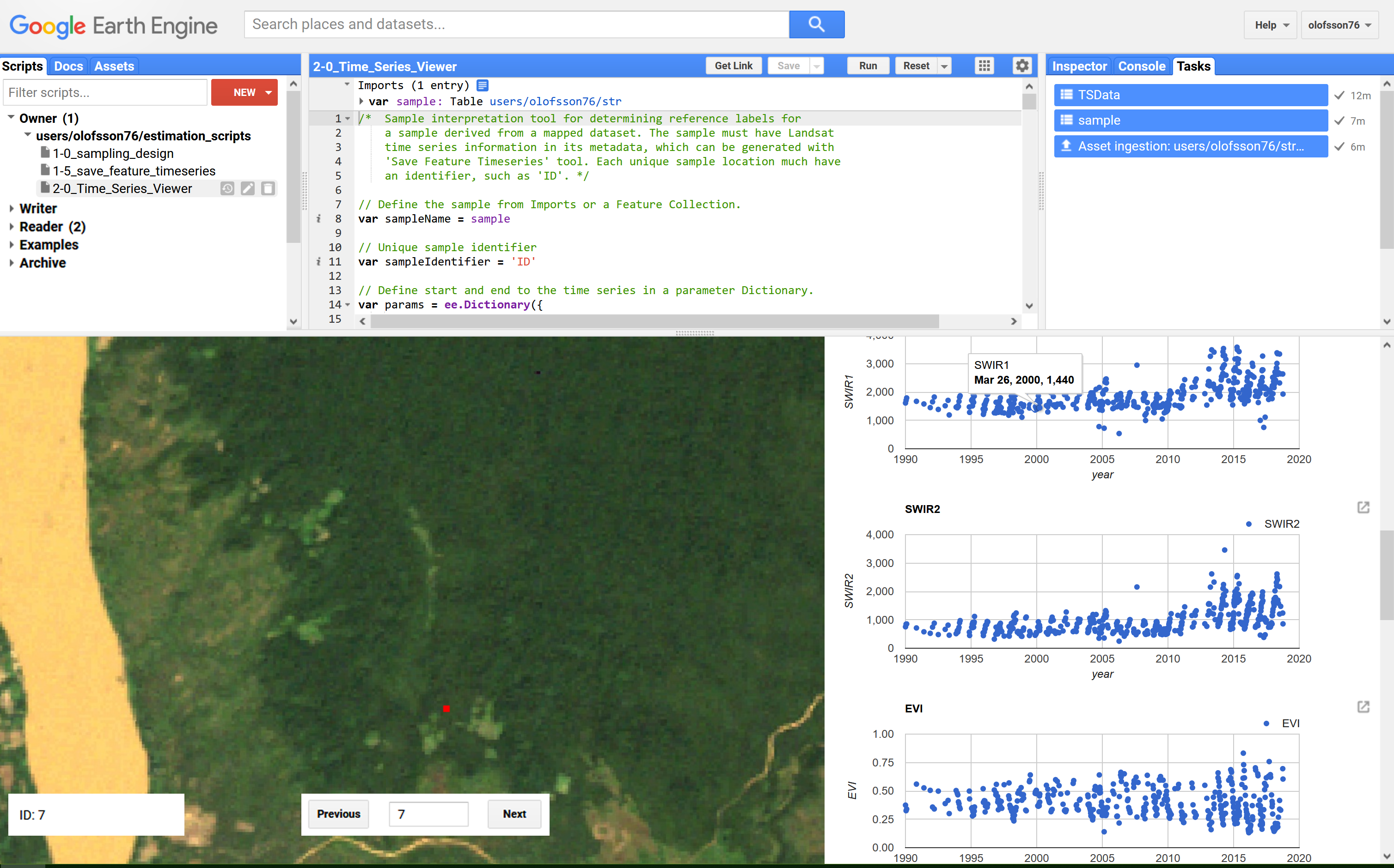
Figure 1. Screen shot of using Time Series Viewer to collect reference observations for sample units.
To record the reference labels, open the CSV file you created in step 2:11 in Google Sheets. Delete columns “classification” and “.geo”.; and add columns “reference”, “reference_name”, “date_event”, “confidence” to the right of column “.geo”.
In column “reference”, record the grid code of the reference label (1: forest, 2: non-forest, 3: water, 4: forest loss, 5: forest gain, and 6: forest loss and gain); in column “reference_name”, write the name of the reference label; in “date_event”, note the year of the loss or gain events; in column “confidence”, indicate by how confident you are that the label is correct – specify 1 if label is uncertain, 2 if probable but not certain, and 3 if certain. For example, I am certain that sample unit #7 in Figure 1 above experienced a forest loss event in 2010. I would then add:
reference: 1
reference_name: Forest loss
date_event: 2010
confidence: 3
Because this is just a tutorial, we won’t go through all sample units. If this was a real life situation though, you would save the CSV after completion as “STR_sample_Cambodia_interpreted.csv” and open it in software that allow you to export the CSV as a shapefile. We recommend using QGIS which executes the GDAL program ogr2ogr – in QGIS, just click Layer > Add Layer > Add Delimited Text Layer; once displayed right-click the CSV file in QGIS layer pane and click Export > Save Feature As; specify ESRI Shapefile as Format and click OK.
- We have prepared a shape file that contains reference labels for each sample unit. Download the following individual files of the shapefile: .prj .shp .shx and .dbf . In Google Earth Engine, click Assets tab > New > Table Upload; navigate to downloaded files and upload the individual .prj .shp .shx and .dbf files of shapefile. Ingesting the shapefile will take about five minutes. The shapefile that contains the sample data should appear in the Assets tab with the name “STR_sample_Cambodia_interpreted” – you are now ready to analyze the sample data.
3. Analysis
- As explained in Choosing an estimator because the sample was selected under stratified random sampling using a categorical change map to define strata, the stratified estimator is efficient for estimating area.
- Run the script 3_0_stratified_estimation. Because we need the strata weights and because we can easily estimate the accuracy of the map using the sample data, under Specify the map used to stratify, specify “stratification_cambodia_utm_small”; specify “reference” under Specify the reference attribute name; and “STR_sample_Cambodia_interpreted” under Specify the reference feature collection – click Load data; and then “Apply stratified estimator”.
- Click Show error matrices to display a cross tabulation of map and reference labels at sample locations. The first matrix shows the number of sample units, \(n_{hj}\) identified as class \(j\) in the reference data in stratum \(h\). The second matrix shows the estimated area proportion of class \(j\) in stratum \(h\) as \(\hat{p}_{hj} = W_h \times n_{hj} \div n_{h+}\).
- The stratification we used doesn’t have a buffer stratum so we won’t click Use buffer stratum. (If the forest loss stratum would have been small and the forest stratum large, it would have been a good idea to create and use a buffer around mapped forest loss.)
- In the Dialog, specify class number “4” (forest loss) under Select map class for which to estimate area and accuracy. This will print the area and accuracy estimates with 95% confidence intervals. Change class to view estimates for the other classes. For Forest loss (class 4), the area ± a 95% confidence interval should be 0.0517 ± 0.0120 expressed as proportion of the total study area or 944,987 ± 219,536 ha. User’s accuracy is 0.62, producer’s 0.80 and overall accuracy 0.92.
| [1] | Hansen, M. C., Potapov, P. V., Moore, R., Hancher, M., Turubanova, S. A. A., Tyukavina, A., … & Kommareddy, A. (2013). High-resolution global maps of 21st-century forest cover change. Science, 342(6160), 850-853. |
| [2] | Cochran, W. G. (1977). Sampling techniques. John Wiley & Sons. |
| [3] | Olofsson, P., Foody, G. M., Herold, M., Stehman, S. V., Woodcock, C. E., & Wulder, M. A. (2014). Good practices for estimating area and assessing accuracy of land change. Remote Sensing of Environment, 148, 42-57. |